
It’s no secret that loading data into a database can be an arduous, time-consuming process. Wouldn’t it be amazing if you could load tens of billions of rows in minutes, instead of hours? With SingleStore, you’ll put slow data ingest behind you. Read on to learn more.
Working with Large Datasets
Have you ever worked with an enormous dataset, something like 50 Million rows? What about 100 million rows? 500 million rows? 1 billion rows? 10 billion rows? How about working with loading and running reports against 100 billion rows in a database table? This might seem like an astronomical number but in today’s world, large datasets are an increasingly realistic scenario for many companies.
In this article, we will show you how to load 100 billion rows at an ultrafast speed in about 10 minutes, resulting in 152.5 million rows per second being ingested into a single database. How? With SingleStore. Just imagine how much value this delivers to your business if you need to load this massive quantity of data in such a short amount of time consistently at regular intervals — whether that’s on a daily, weekly or monthly basis.
A Quick Overview: What Is SingleStore?
SingleStore is a modern, innovative and insanely fast database technology (SQL based) that can ingest, process and perform real-time data analytics. SingleStore is distributed and can easily scale, running on commodity hardware. Our relational database runs all types of workloads including OLTP, DW and HTAP, and is designed to run on-premises, or in hybrid or multi-cloud environments. Overall SingleStore delivers speed, scale and simplicity to power mission-critical and data-intensive applications.
Upload Massively Large Volumes of Data with Pipelines

What are Pipelines?
SingleStore Pipelines are built into our product and are a major differentiator from other database vendors. They allow users to continuously extract, optionally transform and load data in parallel at ultrafast speeds. I’ll dive deeper into how we can create and use Pipelines later in this article — but here are a few key, need-to know Pipeline features:
- Parallel loading, using the full power of a compute cluster
- Support for real-time streaming from files, cloud objects storage and Apache Kafka
- Real-time de-duplication of data
- Support for several data formats such as CSV, JSON, Avro and Parquet
- Support for several data sources including Amazon S3, Azure Blob storage, Google Cloud Storage and HDFS
So, how do we upload 100 billion rows?
Start with SingleStore Cluster
I did the testing for this case using a SingleStore cluster running on our managed service in AWS size (S-32) with the following specifications:
- 3 aggregator nodes(1 master, 2 child)
- 16 leaf nodes
- 128GB of memory per leaf node
- 16 vCPUs(8 CPU cores) per leaf node
- 2TB storage/leaf node
Table structure
We will be loading 100 billion rows into a simple table structure that contains trip information based on the following three integer fields:
- Distance driven in miles
- Duration of the trip in seconds
- Vehicle ID number (unique value)
create table trip_info(distance_miles int, duration_seconds int, vehicle_idint, sort key(distance_miles,duration_seconds));Note in the table structure above we also have a sort key on two columns: distance_miles and duration_seconds. A sort key is a special index that is built on our patented Universal Storage tables. Sort keys allow SingleStore to be data-aware of the column(s) that are indexed, which greatly helps with filtering (segment elimination) and only returns the data needed for the query results.
Another benefit of sort keys is that the data is presorted. An ordered scan over a sort key is faster than sorting a table. Sort keys also benefit from fast joins on columns that have sort keys on them.
Create and start the Pipeline
Using SingleStore Studio (or the command line) we can create the SingleStore Pipeline. The Pipeline syntax specifies the name, directory and location of the AWS S3 bucket folder. We also have the table name we will load the data, specifying the data format delimiter (which is a ‘comma’). The set clause in the Pipeline multiplies the column duration_seconds by 60 to convert the source data from minutes to seconds as we are simultaneously loading data.
CREATE or REPLACE PIPELINE car_trip_details_infoAS LOAD DATA S3 's3://testdata.memsql.com/vehicle_demo2/*'CONFIG '{"region": "us-east-1"} 'INTO TABLE trip_infoFIELDS TERMINATED BY ','(distance_miles, @duration_seconds, vehicle_id)SET duration_seconds = @duration_seconds*60;Starting the pipeline is a straightforward command.
start pipeline car_trip_details_info;Monitor the Pipeline
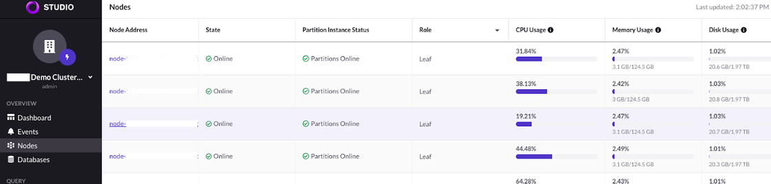
At this point we should be loading data quickly via the SingleStore Pipeline. We can monitor the status of the pipeline by checking the real-time performance from SingleStore Studio. Checking the nodes option on the left-hand side toolbar, we can see CPU, memory and disk activity across all leaf nodes as the data ingestion is in progress.
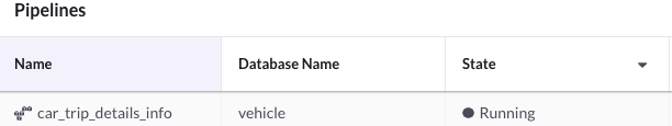
You can verify a Pipeline status in SingleStore Studio by clicking the Pipelines option located on the lower left-hand side of the screen, then check the “State” column. In this example, the “State” is shown as “Running”.
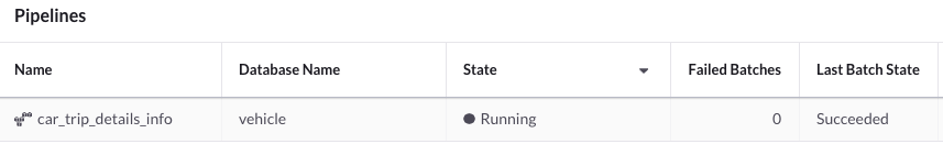
The example screenshot here shows a completed Pipeline with the “Last Batch State” column having the value of “Succeeded”.
The command you see here returns the status of the current load stream, duration in seconds and the number of rows loaded or streamed into the database.
We may also get multiple rows returned — and once all rows show the value as “Succeeded,” then the Pipeline has completed loading all of the data from our CSV files.
select batch_state, batch_time, rows_streamed frominformation_schema.pipelines_batches_summary where database_name = "vehicle";Verify the loaded data
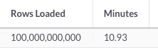
The SQL statement below returns the total numbers of rows loaded and the duration in minutes.
select format(sum(rows_streamed),0) "Rows Loaded",round(sum(batch_time)/60,2)"Minutes" from information_schema.pipelines_batches_summary;The screenshot below from SingleStore Studio highlights the output from loading 100 billion rows in 10.93 minutes — just as we teased at the beginning of our article.
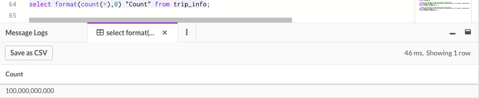
Now, let’s count the rows in the table. As you can see from this screenshot, we counted 100 billion rows in just 46 milliseconds. And SingleStore consistently delivers this impressive display of speed.
Data distribution
This table shows the data distributed in the trip_info table that was loaded by the SingleStore Pipeline. We have 10 rows, each with a unique vehicle_id and the count of entries the specific vehicle appears within the trip table. For example: In the first row, vehicle_id 6 appears in the tripinfo table 34,475,000,000 times, whereas for _vehicle_id 7 occurs 1,475,000,000 times. The total input row count is 100 billion.
| 6 | 35,475,000,000 |
| 9 | 20,475,000,000 |
| 8 | 10,475,000,000 |
| 4 | 8,475,000,000 |
| 3 | 7,975,000,000 |
| 1 | 5,475,000,000 |
| 10 | 5,475,000,000 |
| 2 | 2,975,000,000 |
| 5 | 1,725,000,000 |
| 7 | 1,475,000,000 |
| Total Input rows | 100,000,000,000 |
Let’s revisit the question I first asked at the beginning of this article: How would ultrafast data ingest and loading benefit your business? We can think of a few ways. If you’re ready to try it out for yourself, check out the free Singlestore Helios trial today.
Appendix
Data creation process
We create a Unix shell script to accomplish this task.
#!/bin/bash

total_times=147500000

# duration in minutes to drive 1 mile
time_for_mile=1

for milesdriven in 1 5 10 25 50 75 100 125 150 175
{
export distance_traveled=`echo $time_for_mile \* $milesdriven | bc -l`
for ((i=1; i <= $total_times; i=i+1))
   do
    echo $milesdriven,$distance_traveled,"7"
   done
}
The script above starts by setting a variable total_times — this will be used within a loop and will be explained later. The next variable is time_for_mile: this represents the amount of time it takes a vehicle to drive one mile. Subsequently, we start an outer for loop and iterate through 10 values of the variable milesdriven (note this loop only executes 10 times since we have 10 values).
Next, we calculate the value for the variable distance_traveled, which is simply multiplying the variables time_for_value by milesdriven. Finally, we enter into the next inner “for loop” and execute it 147,500,000 times (this is the value of the variable total_times that we referenced earlier). Consider the total number of resulting rows will be 10 multiplied by the value of the variable total_times, so in this example we will get 1,475,000,000 — or 1.475 Billion rows.
I created a total of 10 unique scripts and within each script, there are three differences (colored green in the accompanying script screenshot ) for the settings of the variables time_for_mile, total_times and the value of the vehicle_id which is the third field in the echo command (in this case it is 7).
In my case for each vehicle_id, I set the value for the variable total_times to be 10 times smaller than the expected resulting rows, shown in the table below. Notice the total rows created are 100 billion, spanning 10 output files. Each file represents a vehicle that has varying amounts of rows, from 147.5 million to around 35.5 billion.
Please note: generating 100 billion rows across the 10 output files may take 2-3 days. Ideally it would be best to run the scripts on a server with the processing capacity to handle this large workload. In my case, the server I ran the load script from has the following specifications:
- EC2 instance(VM) on AWS.
- Chip type Intel(R) Xeon(R) Platinum 8259CL CPU @ 2.50GHz
- 2 CPU sockets, 24 CPU cores per socket, 48 total CPU cores, 64 vCPUs
- 384GB of Memory
- Storage SSD IO2, max IOPS setting 16,000
Next, we invoke a master shell script that will execute all 10 shell scripts in parallel, also in the background and in nohup mode.
nohup ./gen_data_vehicle1.sh > vehicle1 &nohup ./gen_data_vehicle2.sh > vehicle2 &nohup ./gen_data_vehicle3.sh > vehicle3 &nohup ./gen_data_vehicle4.sh > vehicle4 &nohup ./gen_data_vehicle5.sh > vehicle5 &nohup ./gen_data_vehicle6.sh > vehicle6 &nohup ./gen_data_vehicle7.sh > vehicle7 &nohup ./gen_data_vehicle8.sh > vehicle8 &nohup ./gen_data_vehicle9.sh > vehicle9 &nohup ./gen_data_vehicle10.sh > vehicle10 &In retrospect, I could have created one master script and simply imported the values of the variables as arguments on the command line to avoid having 10 different scripts.
Prepare the data files
SingleStore Pipelines work very well to load multiple files in parallel. In our case once we have all 10 output files created, then we will split each individual file into 10 pieces resulting in 100 files for each vehicle for a total of 1,000 files. I did testing with various CSV files to load, and found the sweet spot was 1,000 files for my particular use case. The following script shows I used the Unix split command to break each CSV file into smaller pieces.
nohup split -l 54750000 vehicle1 vehicle1z_ &nohup split -l 29750000 vehicle2 vehicle2z_ &nohup split -l 79750000 vehicle3 vehicle3z_ &nohup split -l 84750000 vehicle4 vehicle4z_ &nohup split -l 17250000 vehicle5 vehicle5z_ &nohup split -l 354750000 vehicle6 vehicle6z_ &nohup split -l 14750000 vehicle7 vehicle7z_ &nohup split -l 104750000 vehicle8 vehicle8z_ &nohup split -l 204750000 vehicle9 vehicle9z_ &nohup split -l 54750000 vehicle10 vehicle10z_ &Next I compress all 1,000 files using the gzip command. The total space consumed by all 1,000 compressed files is only 2.0GB. To save time I wrote a simple shell script to gzip all 1,000 files simultaneously in the background.
Once all of the CSV files are compressed, then I copied them to an online folder in an AWS S3 bucket. Lastly, I verified all 1,000 compressed files are in the AWS S3 bucket folder.